In this post, I review Locality-Sensitive Hashing for near-duplicate detection. I demonstrate the principle and provide a quick intro to Datasketch which is a convenient library to run near-duplicate detection at scale.
The problem being solved
Once I needed to find near-duplicates in a (relatively) large collection of texts ~5 mln. docs. I wanted the solution to be:
- easy-to-use
- scalable
- exact, i.e. when a pair of near-duplicate texts is flagged, we can be confident that those are indeed near-duplicates.
I somehow struggled for quite a while to find a solution that would satisfy all conditions. Until I found Locality-Sensitive Hashing (LSH) and its implementation – Datasketch.
MinHash LSH – the principle
1. When we need to deduplicate a single dataset

In a nutshell, this works as follows. For a most typical scenario where we need to identify near-duplicates in a single collection of texts, we perform the following steps:
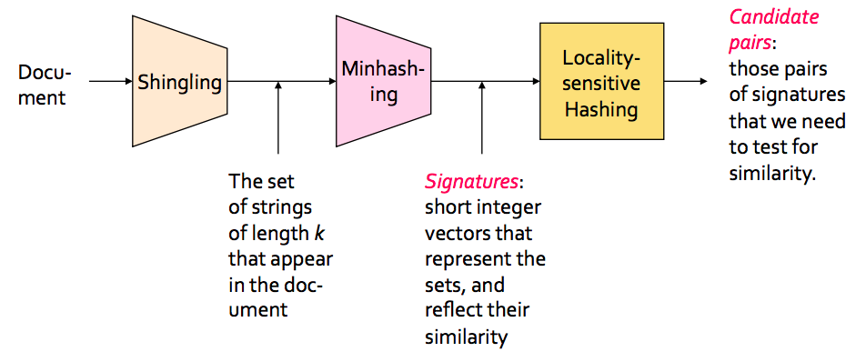
- the text is processed and cut into shingles (overlapping substrings of a fixed size);
- then a set of shingles is minhashed, this involves creating multiple hashes for a set of shingles, so that we end up with a single vector of integers for each piece of text, a.k.a. a signature;
- the dimension of the hash vector is further reduced via Locality-Sensitive Hashing, which is creating a single hash from a number (band) of nearby elements in the hash vector. The resulting vector is also called a bandhash signature or bandhash vector;
- all pairs of signatures where elements match at least in one position, generate candidate pairs;
- (optionally) we can measure the true similarity between corresponding pieces of text to account for errors (False Positives) of the LSH algorithm.
I know there are quite a few terms here. Instead of explaining all of them (and thus re-writing something similar to this nice blog post) I’d refer to a classical book “Mining massive datasets”, ch. 3 for an intro into Locality-Sensitive Hashing and finding similar items. In this blog post, we’ll focus on a practical use case of finding near-dups in a large collection of texts.
2. When we have incoming “query” data that we want to compare to a large “index” dataset
Here “historical” data can be a large dataset, e.g. 5 mln. documents.
The “query” dataset is much smaller, e.g. 10K documents that we receive daily, say via some API, and would like to deduplicate.

We can do without LSH at all just comparing 10K fresh documents to 5 mln. historical documents. But that’d require 50 bln. comparisons each day might be too computationally prohibitive (a dumb idea leading, above all, to a considerable carbon footprint). LSH is a technique that approximates the exact similarity function.
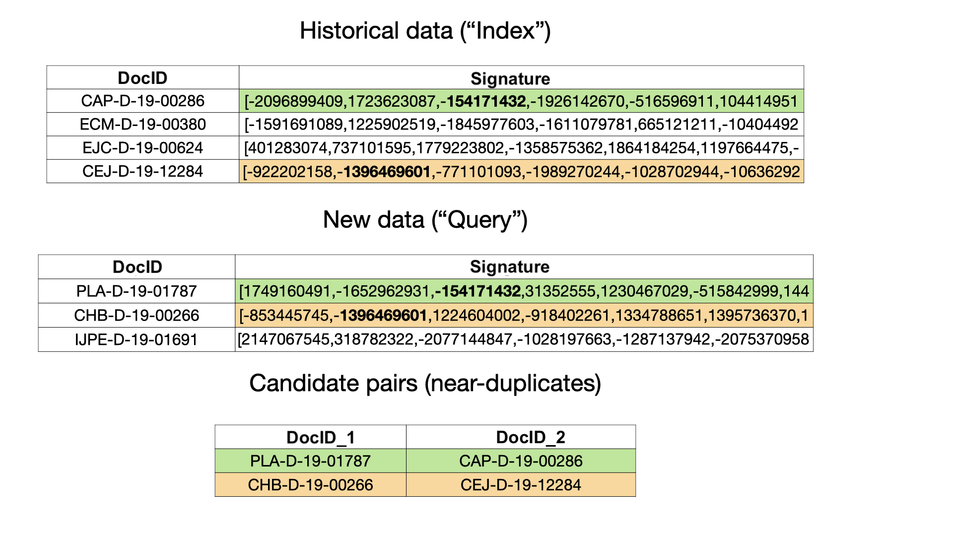
The essence of the algorithm is to create signatures for each piece of text that is identified here by a DocID. Signatures are just numeric vectors of some fixed dimension, e.g. 128.
For two pieces of text to be considered as candidates for near-duplicates, it suffices for their hash signatures to match in at least one component. In the picture above, a pair highlighted in green is a candidate, and a pair highlighted in orange is another one. Bolded are those matching hash values.
Limitations
- The method only takes care of the lexical similarity not semantical. Thus, with LSH, we won’t identify near-duplicates that differ due to parapharasing, synonym replacement, etc.
- The method is probabilistic, i.e. some errors are allowed. Not all candidates would actually be near-duplicates. One can check this by calculating Jaccard similarity of the candidates. Thus, the algorithm is characterized by precision (out of all pairs of candidates found by the algorithm, what’s the proportion of real near-duplicates, i.e. with their Jaccard similarity exceeding the predefined threshold) and recall (out of all near-duplicate pairs, what’s the proportion of those found by the algorithm).
- In practice, for a large enough dataset and long pieces of text (e.g. full documents not just titles), LSH tends to work worse in terms of precision while recall can not be known without a crazy carbon footprint. Finding true near-duplicate pairs in a relatively small collection of 50K texts requires >1.2B calls to a Jaccard similarity subroutine.
# imports
import json
import pickle
import re
from pathlib import Path

import numpy as np
import pandas as pd
from datasketch import MinHash, MinHashLSH
from matplotlib import pyplot as plt
from num2words import num2words
from tqdm import tqdm
Preprocessing and hashing
Essentially, MinHashLSH operates with shingle sets where shingles are overlapping substrings of a fixed size. The following 4 code cells show how MinHashLSH builds hash vectors (a.k.a. Signatures) for entry texts.
Further, as described in the picture above, for two pieces of text to be considered as candidates for near-duplicates, it suffices for their hash signatures to match in at least one component
s = "this is a piece of text"
shingle_size = 4

shingle_set = {s[i : i + shingle_size]
               for i in range(len(s) - shingle_size + 1)}
shingle_set
{' a p',
 ' is ',
 ' of ',
 ' pie',
 ' tex',
 'a pi',
 'ce o',
 'e of',
 'ece ',
 'f te',
 'his ',
 'iece',
 'is a',
 'is i',
 'of t',
 'piec',
 's a ',
 's is',
 'text',
 'this'}
def hash_func(a_string, salt: int = 1):
    return hash(a_string + str(salt))
These are the 5 components of a toy 5-dimensional hash signature. Each one of them is created by hashing all shingles and taking a min. value of the hashes.
for i, salt in enumerate(range(5)):
    print(i, min([hash_func(el, salt=salt) for el in shingle_set]))
0 -7220920153181112185
1 -9127360350460247126
2 -8803612098918371157
3 -8027849914885749588
4 -9069105076530742277
Datasketch LSH – a toy example
from datasketch import MinHash, MinHashLSH
SIMILARITY_THRESHOLD = 0.6
NUM_PERMS = 96
SHINGLE_SIZE = 4
Three similar strings. We’ll index first two, and then look for near-duplicates for the 3rd one.
s1 = "This is a piece of text"
s2 = "This is a similar piece of text"
s3 = "This is also a similar piece of text"
Inserting strings split by whitespaces into MinHash objects.
minhash1 = MinHash(num_perm=NUM_PERMS)
minhash2 = MinHash(num_perm=NUM_PERMS)
minhash3 = MinHash(num_perm=NUM_PERMS)

for d in set(s1.split()):
    minhash1.update(d.encode("utf8"))
for d in set(s2.split()):
    minhash2.update(d.encode("utf8"))
for d in set(s3.split()):
    minhash3.update(d.encode("utf8"))
Create LSH index and insert first 2 MinHashobjects in it.
lsh = MinHashLSH(threshold=SIMILARITY_THRESHOLD, num_perm=NUM_PERMS)
lsh.insert("text1", minhash1)
lsh.insert("text2", minhash2)
Querying near-duplicates for the 3rd piece of text.
lsh.query(minhash3)
['text2'
Same with Redis storage as a backend, not Python dictionaries
See MinHashLSH docs to configure the algo to run with the Redis backend. The idea is that to query LSH for near-duplicates, we only need to make lookups to get signatures. Redis is an in-memory database that allows for very fast lookups, also, it scales much better than Python dictionaries.
lsh_redis = MinHashLSH(
    threshold=SIMILARITY_THRESHOLD,
    num_perm=NUM_PERMS,
    storage_config={"type": "redis",
                    "redis": {"host": "localhost",
                              "port": 6379}},
)
lsh_redis.insert("text1", minhash1)
lsh_redis.insert("text2", minhash2)
lsh_redis.query(minhash3)
['text2']
Running LSH near-duplicate detection with a real-world dataset
Further, we run the algorithm with some realistic dataset – news about cryptocurrencies, Kaggle dataset.
SIMILARITY_THRESHOLD = 0.8
NUM_PERMS = 128
SHINGLE_SIZE = 4
lsh = MinHashLSH(threshold=SIMILARITY_THRESHOLD, num_perm=NUM_PERMS)
Reading data
# You can download the dataset and customize this path
PATH_TO_DATA = Path("crypto_news")
The following two parts of the dataset would imitate the historical part (index_df) and the query part (query_df). For each title in the qury part, we’d like to find near-duplicate titles in the historical part.
index_df = pd.read_csv(PATH_TO_DATA /
                       "crypto_news_parsed_2013-2017_train.csv")
query_df = pd.read_csv(PATH_TO_DATA /
                       "crypto_news_parsed_2018_validation.csv")
We’ll identify each title by some id, so reindexing. Also, there are quite a few fields in the dataset, we’ll take care only of the title field.
index_df.index = [f'train_{i}' for i in range(len(index_df))]
query_df.index = [f'val_{i}' for i in range(len(query_df))]
index_df[['title']].head(2)
| title | |
|---|---|
| train_0 | Bitcoin Price Update: Will China Lead us Down? |
| train_1 | Key Bitcoin Price Levels for Week 51 (15 – 22 ... |
query_df[['title']].head(2)
| title | |
|---|---|
| val_0 | Paris Hilton’s Hotel Mogul Father to Sell $38 ... |
| val_1 | Playboy Sues Cryptocurrency Company for Breach... |
def preprocess(string, maxlen=500):
    tmp_string = string[:maxlen]
    tmp_string = re.sub(r"(\d+)",
                        lambda x: num2words(int(x.group(0))),
                        tmp_string)
    res = re.sub(r"[\W]+", "", tmp_string).lower()
    return res


def _shingle(string, shingle_size=4):
    shings = {
        string[i : i + shingle_size]
        for i in range(len(string) - shingle_size + 1)
    }
    return set(shings)
LSH from Datasketch
lsh = MinHashLSH(threshold=SIMILARITY_THRESHOLD, num_perm=NUM_PERMS)
Populating the index
for id_, title in tqdm(index_df['title'].iteritems()):

    title_shingles = _shingle(preprocess(title),
                              shingle_size=SHINGLE_SIZE)

    title_minhash = MinHash(num_perm=NUM_PERMS)

    for shing in title_shingles:
        title_minhash.update(shing.encode("utf8"))

    lsh.insert(id_, title_minhash, check_duplication=False)
We’ve indexed that many titles:
len(lsh.get_counts()[0])
27462
If needed, we can serialize the LSH object
with open("lsh.pkl", "wb") as f:
    pickle.dump(lsh, f)
!du -hc lsh.pkl
 35M	lsh.pkl
 35M	total
Get near-duplicates for the query data
dup_dict = {}

for id_, title in tqdm(query_df['title'].iteritems()):

    title_shingles = _shingle(preprocess(title),
                              shingle_size=SHINGLE_SIZE)

    title_minhash = MinHash(num_perm=NUM_PERMS)

    for shing in title_shingles:
        title_minhash.update(shing.encode("utf8"))

    dups = lsh.query(title_minhash)
    dup_dict[id_] = dups
(Optional step) Analyze true Jaccard similarity
def jaccard_similarity(list1, list2):
    s1 = set(list1)
    s2 = set(list2)
    return len(s1.intersection(s2)) / len(s1.union(s2))
To access precision, we calculate the actual Jaccard similarity for the candidates identified by LSH.
jaccard_sims = []

for id_, dups in tqdm(dup_dict.items()):
    if dups:
        shingle_query_title = _shingle(
                              preprocess(
                              query_df.loc[id_, "title"]))
        for dup_id in dups:
            shingle_indexed_title = _shingle(
                                     preprocess(
                                     index_df.loc[dup_id, "title"]))
            sim = jaccard_similarity(
            	shingle_query_title,
            	shingle_indexed_title)
            jaccard_sims.append(sim)
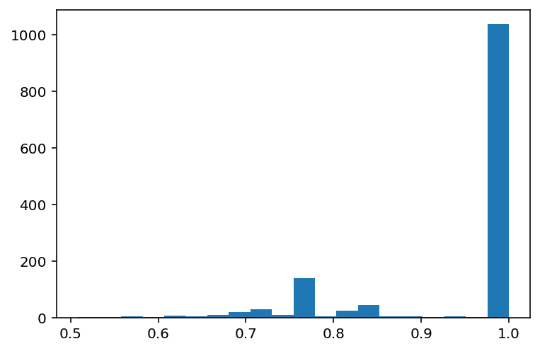
plt.hist(jaccard_sims, bins=20);

The distribution is nice, mostly, LSH indeed captures similar pairs.
Precision
(pd.Series(jaccard_sims) >= SIMILARITY_THRESHOLD).sum() / len(jaccard_sims)
0.8334
NOTE: That’s the precision of the LSH algorithm. In practice, it’s very easy to have 100% precision with an additional effort of calculating the actual Jaccard similarity for the candidate pairs (as done above) and filtering out false positives, i.e. the candidates pairs with similarity below the predefined threshold.
Recall
This is a very computationally intensive step (that we are speeding up with multiprocessing) – we calculate all pairwise Jaccard similarities between 11k query titles and 27k indexed titles and see how many true near-duplicates the LSH algo missed.
shingled_query_text = [
    _shingle(preprocess(el)) for el in tqdm(query_df["Title"])
]
shingled_index_texts = [
    _shingle(preprocess(el)) for el in tqdm(index_df["Title"])
]
Building pairwise Jaccard similarity matrix with multiprocessing
from multiprocessing import Pool

class JaccardPool(object):
    def __init__(self, archive_shingles):
        self.archive_shingles = archive_shingles

    def __call__(self, val_shing):
        """
        :param val_shing: a shingle set to compare with each one in
                          `archive_shingles` and to calculate Jaccard similarity
        """
        return [
            jaccard_similarity(val_shing, arch_shing)
            for arch_shing in self.archive_shingles
        ]
try:
    pool = Pool(8)  # on 8 processors
    engine = JaccardPool(archive_shingles=shingled_index_texts)
    sims = pool.map(engine, shingled_query_text)
finally:  # To make sure processes are closed in the end, even if errors happen
    pool.close()
    pool.join()
Now we have a similarity matrix of size [11k, 27k] which we can use to compute recall, i.e. how many pairs with Jaccard similarity over the given threshold we managed to find.
sim_matrix = np.vstack(sims)
print((pd.Series(jaccard_sims) >= SIMILARITY_THRESHOLD).sum() /
      (sim_matrix >= SIMILARITY_THRESHOLD).sum())
0.925
NOTE: We see that with short titles recall is pretty high. In reality though, for large datasets, recall is unknown (without a crazy carbon footprint from computing all pairwise text similarities).
Literature
- “Mining massive datasets”, ch. 3 – the theoretical foundation of Locality-Sensitive Hashing
- A blog post on this topic
- Datasketch – a Python library implementing, among all, the
MinHashLSHalgorithm